Cell Type Deconvolution for High-Resolution Slide-seq Colorectal Cancer

Python GPU-accelerated Adapted from the SpaCET R tutorial for colorectal cancer Slide-seq

Overview

This tutorial demonstrates how to use spatial-gpu to deconvolve high-resolution spatial transcriptomics data from a colorectal cancer (CRC) sample profiled using the Slide-seq platform (Zhao et al., 2021). Each 10 μm bead captures approximately 1–2 cells, providing near single-cell resolution.

The high-resolution nature of Slide-seq data means that each bead is expected to contain at most 1–2 cells, making the deconvolution problem different from lower-resolution platforms like Visium (~55 μm) or oldST (~100 μm). The SpaCET algorithm handles this by adapting its cell fraction estimation to the platform resolution.

The spatial-gpu package provides a GPU-accelerated Python implementation of the SpaCET algorithm (Nature Communications 14, 568, 2023). All functions work on AnnData objects and store results in adata.uns['spacet'].

API Mapping: R SpaCET → spatial-gpu

1. Create SpaCET Object

Load the CRC Slide-seq data into an AnnData object. The dataset contains 10 μm beads with spatial coordinates and gene expression counts.

import spatialgpu.deconvolution as spacet
import anndata as ad

# Load Slide-seq CRC data from h5ad file
adata = ad.read_h5ad("data/hiresST_CRC/hiresST_CRC.h5ad")

# Inspect the object
print(adata)

2. Deconvolve ST Data

Run the two-stage SpaCET deconvolution algorithm for colorectal cancer. Stage 1 estimates the malignant cell fraction using CRC-specific copy number alteration and expression signatures. Stage 2 decomposes the non-malignant fraction into immune and stromal cell types using hierarchical constrained regression.

# Run two-stage deconvolution for colorectal cancer (CRC)
adata = spacet.deconvolution(adata, cancer_type="CRC", n_jobs=6)

# View deconvolution results (cell types x spots)
prop_mat = adata.uns['spacet']['deconvolution']['propMat']
print(f"Cell types: {prop_mat.shape[0]}")
print(f"Beads: {prop_mat.shape[1]}")
print(prop_mat.iloc[:, :6])

3. Visualize Results

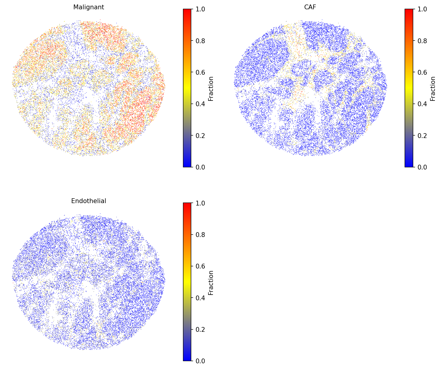
3a. Cell type fractions

Visualize selected cell-type fractions across the tissue. Use a smaller point_size to accommodate the high density of Slide-seq beads.

# Visualize selected cell type fractions
spacet.visualize_spatial_feature(
    adata,
    spatial_type="CellFraction",
    spatial_features=["Malignant", "CAF", "Endothelial"],
    point_size=0.6,
    same_scale_fraction=True,
)

Spatial distribution of Malignant, CAF, and Endothelial cell fractions in the CRC Slide-seq dataset. Color scale: blue (low) → yellow → red (high). Malignant cells cluster in the tumor core, while CAF and Endothelial cells are enriched in the stroma.

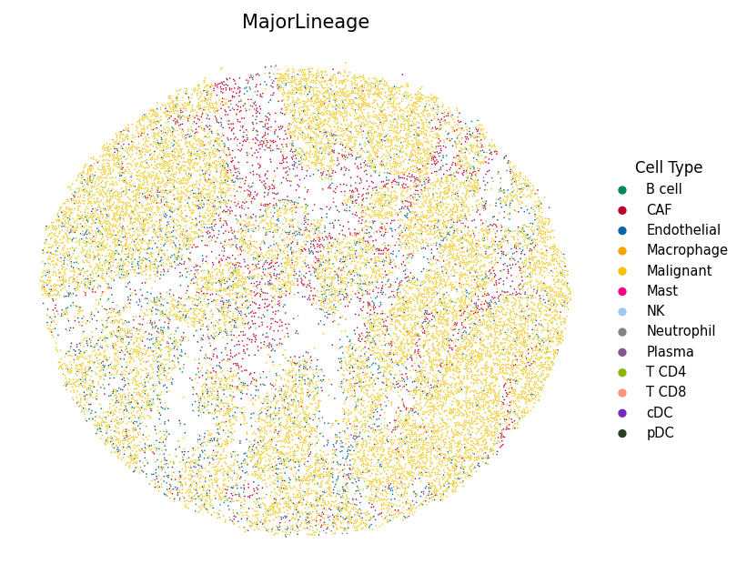
3b. Most abundant cell type

Assign each bead to its dominant cell type and display with custom colors to highlight the spatial organization of the tumor microenvironment.

import json

# Load color mapping (matching R tutorial's colors_vector.rda)
with open("data/hiresST_CRC/colors_vector.json") as f:
    colors_vector = json.load(f)

# Visualize the most abundant cell type per bead
spacet.visualize_spatial_feature(
    adata,
    spatial_type="MostAbundantCellType",
    spatial_features=["MajorLineage"],
    colors=colors_vector,
    point_size=0.6,
)

Each bead colored by its dominant cell type. The high resolution of Slide-seq reveals fine-grained spatial organization of the tumor microenvironment, with clear boundaries between malignant and stromal regions.

Session Info

import spatialgpu
print(f"spatial-gpu version: {spatialgpu.__version__}")

import anndata, numpy, scipy, pandas, matplotlib
print(f"anndata:     {anndata.__version__}")
print(f"numpy:       {numpy.__version__}")
print(f"scipy:       {scipy.__version__}")
print(f"pandas:      {pandas.__version__}")
print(f"matplotlib:  {matplotlib.__version__}")

try:
    import cupy
    print(f"cupy:        {cupy.__version__} (GPU backend available)")
except ImportError:
    print("cupy:        not installed (CPU-only mode)")