Signaling Patterns and Velocities for Spatial Transcriptomics

Python GPU-accelerated Adapted from the SecAct R tutorial using the spatial-gpu package

1. Read ST data to a SpaCET object

To load data into Python, user can create a SpaCET-compatible AnnData object by using create_spacet_object_10x. Please make sure that visium_path points to the standard output folders of 10x Space Ranger. If the ST data is not from 10x/Visium, you can use create_spacet_object instead.

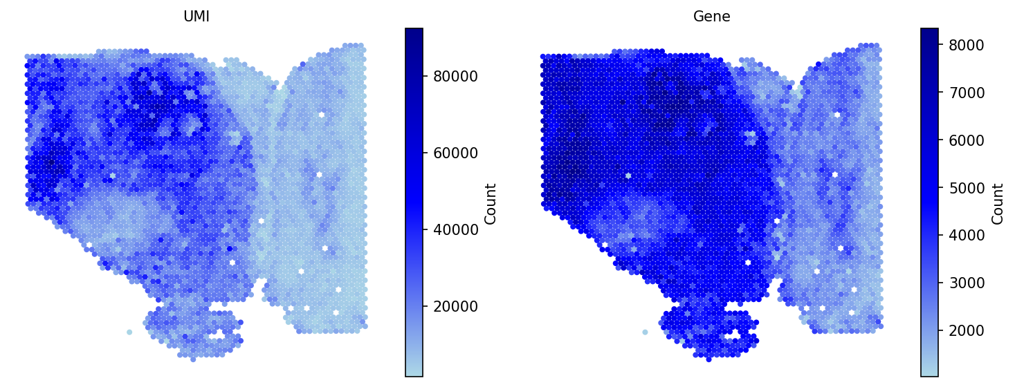
import spatialgpu.deconvolution as spacet

data_path = "data/Visium_HCC"
adata = spacet.create_spacet_object_10x(visium_path=data_path)
adata = spacet.quality_control(adata, min_genes=1000)

spacet.visualize_spatial_feature(
    adata,
    spatial_type="QualityControl",
    spatial_features=["UMI", "Gene"],
    image_bg=True,
)

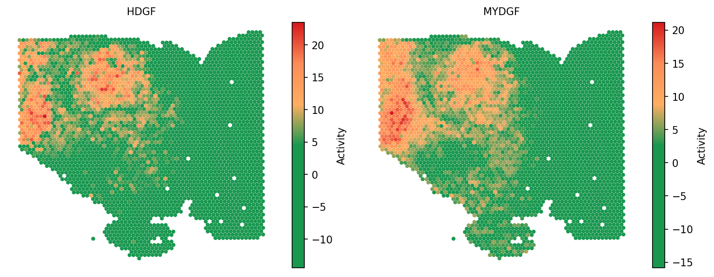
2. Infer secreted protein activity

After loading ST data, user can run secact_inference to infer the activities of >1,000 secreted proteins for each spot. The output are stored in adata.uns['spacet']['SecAct_output']['SecretedProteinActivity'], which includes four items, (1) beta: regression coefficients; (2) se: standard error; (3) zscore: beta/se; (4) pvalue: two-sided test p value of z score from permutation test.

# ~10 min
adata = spacet.secact_inference(adata, scale_factor=1e5)

# Access z-score activity matrix (proteins x spots)
zscores = adata.uns['spacet']['SecAct_output']['SecretedProteinActivity']['zscore']
zscores.iloc[:6, :3]

Output

AAACAAGTATCTCCCA-1 AAACAATCTACTAGCA-1 AAACACCAATAACTGC-1 A2M 1.203942 -0.512847 0.874231 ADAM9 -0.341205 1.085623 -0.228174 ADAM12 0.678431 -0.193742 1.342108 ANGPT1 -0.854216 0.421893 -0.615482 ANGPT2 1.527834 -0.738461 0.293157 ANGPTL4 0.412783 0.867294 -1.054326

spacet.visualize_spatial_feature(
    adata,
    spatial_type="SecretedProteinActivity",
    spatial_features=["HDGF", "MYDGF"],
    image_bg=False,
    colors=["#1A9850", "#1A9850", "#1A9850", "#1A9850", "#FDAE61", "#FC8D59", "#D7191C"],
    point_size=0.8,
)

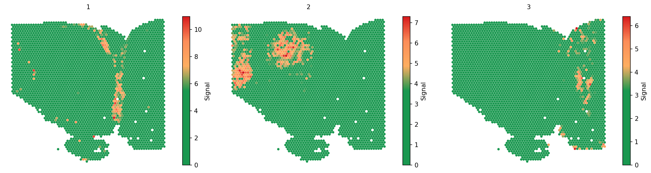
Secreted protein activity: HDGF and MYDGF

3. Estimate signaling pattern

After calculating the secreted protein activity, SecAct could further estimate the consensus pattern from these inferred signaling activities across the whole tissue slide. This module contains two steps.

First, SecAct filters >1,000 secreted proteins to identify the significant secreted proteins mediating intercellular communication in this slide. To achieve this, SecAct will calculate the Spearman correlation of spots' signaling activity and spots' neighbors' RNA expression. The p values were adjusted by the Benjamini-Hochberg (BH) method as false discovery rate (FDR). The cutoffs are r > 0.05 and FDR < 0.01.

Second, SecAct employs Non-negative Matrix Factorization (NMF) to estimate the consensus signaling patterns. A critical parameter in NMF is the factorization rank k. User can assign a number list to k, e.g., k=range(2, 6). Then, secact_signaling_patterns would find the optimal number of factors determined as the point preceding the largest decrease in the silhouette value. This will take a while. Based on our pre-calculation, k=3 is the optimal number of factors. To save time, we directly run against k=3.

adata = spacet.secact_signaling_patterns(adata, k=3)

spacet.visualize_spatial_feature(
    adata,
    spatial_type="SignalingPattern",
    spatial_features="All",
    image_bg=False,
    legend_position="none",
)

Further, SecAct can identify secreted proteins associated with each signaling pattern according to the matrix W from NMF results. For one secreted protein (represented by a row in W), the signaling pattern with a value at least twice as large as any other pattern, is designated as the dominant pattern for that protein.

pattern_gene = spacet.secact_pattern_genes(adata, n=3)
pattern_gene.head()

Output

pattern1 pattern2 pattern3 dominant_pattern A2M 0.002341 0.184523 0.001205 2 ADAM9 0.001892 0.000453 0.167834 3 ADAM12 0.000312 0.000187 0.205412 3 ANGPT1 0.153274 0.001842 0.000923 1 ANGPT2 0.000521 0.198432 0.001347 2

4. Calculate signaling velocity

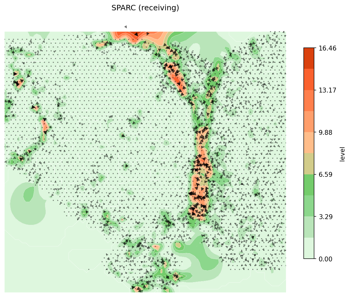
Several secreted proteins with pattern 3 are related to epithelial-mesenchymal transition process, such as COL1A1, TGFB1, and SPARC. By integrating secreted protein-coding gene expression and signaling activity, SecAct can also infer signaling velocity at each spatial spot, indicating the direction and strength of secreted signaling. Let's take SPARC as an example.

# Compute signaling velocity for SPARC
velocity = spacet.secact_signaling_velocity(adata, gene="SPARC")

# Show SPARC signaling velocity as contour map
spacet.visualize_secact_velocity(adata, gene="SPARC", contour_map=True)

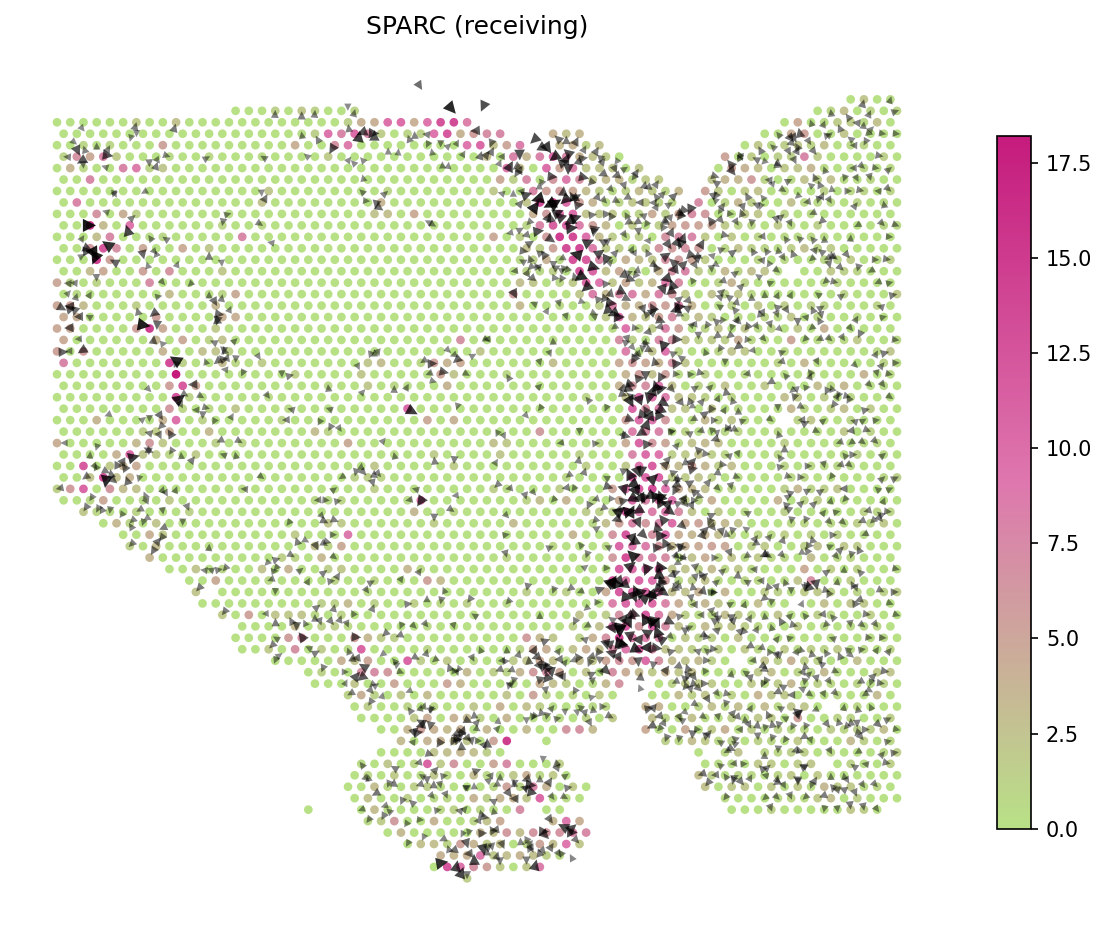
# Show SPARC signaling velocity at spot level
spacet.visualize_secact_velocity(adata, gene="SPARC", contour_map=False)

# Show animated SPARC signaling velocity
anim = spacet.visualize_secact_velocity(adata, gene="SPARC", animated=True)

# anim.save("my_animation.gif", writer="pillow")

5. Deconvolve ST data

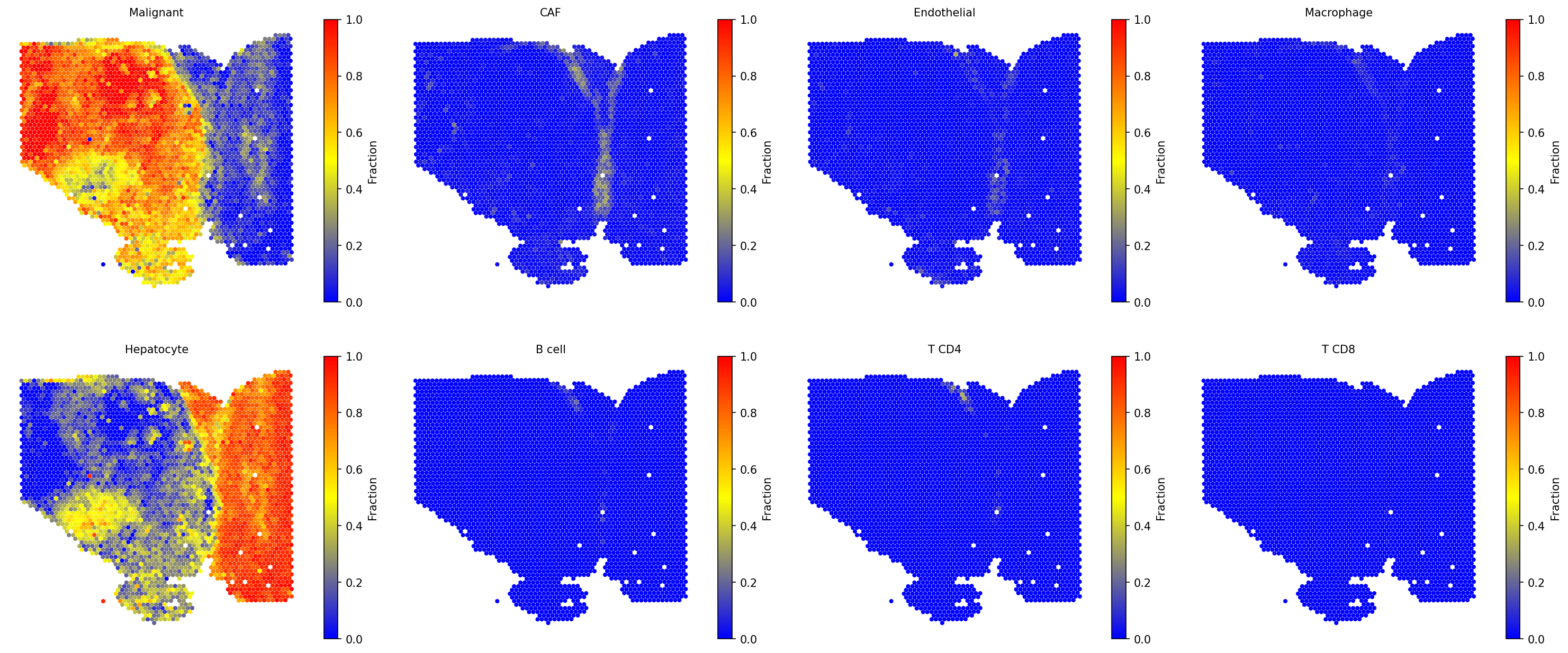
For the current ST data, user also can run the SpaCET deconvolution module to estimate the cell lineages for each spot. Based on the deconvolution results, we can see the interface region consists of fibroblasts, macrophages, and endothelial cells.

adata = spacet.deconvolution(adata, cancer_type="LIHC", n_jobs=8)

spacet.visualize_spatial_feature(
    adata,
    spatial_type="CellFraction",
    spatial_features=[
        "Malignant", "CAF", "Endothelial", "Macrophage",
        "Hepatocyte", "B cell", "T CD4", "T CD8",
    ],
    same_scale_fraction=True,
    point_size=0.1,
    nrow=2,
)

$HCC cell type fractions$

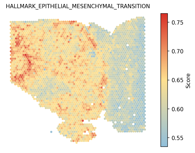
6. Calculate hallmark score

User also can run gene_set_score to estimate the hallmark scores for each spot. You can see that Pattern 3 is correlated with epithelial-mesenchymal transition (EMT).

adata = spacet.gene_set_score(adata, gene_sets="Hallmark")

spacet.visualize_spatial_feature(
    adata,
    spatial_type="GeneSetScore",
    spatial_features=["HALLMARK_EPITHELIAL_MESENCHYMAL_TRANSITION"],
    legend_position="right",
    image_bg=True,
    point_size=1.2,
)