Cell Type Deconvolution and Cell-Cell Interaction Analysis for Visium Breast Cancer

Python GPU-accelerated Adapted from the SpaCET R tutorial using the spatial-gpu package

Overview

This tutorial demonstrates how to use spatial-gpu to estimate cell-type identities and cell-cell interactions in spatial transcriptomics data. We use a 10x Visium breast cancer dataset where each 55 μm spot captures approximately 1–10 cells.

The spatial-gpu package provides a GPU-accelerated Python implementation of the SpaCET algorithm (Nature Communications 14, 568, 2023). All functions in this tutorial work on AnnData objects and store results in adata.uns['spacet'].

The Visium breast cancer dataset is available from 10x Genomics.

API Mapping: R SpaCET → spatial-gpu

1. Create SpaCET Object

Load the 10x Visium breast cancer data into an AnnData object. The function reads the Space Ranger output directory containing the filtered feature-barcode matrix and spatial information. Spot IDs are formatted as "{array_row}x{array_col}".

import spatialgpu.deconvolution as spacet

# Path to Space Ranger output directory
visium_path = "data/Visium_BC"

# Create AnnData object from 10X Visium data
adata = spacet.create_spacet_object_10x(visium_path)

# Inspect the object
print(adata)
print(adata.X[:8, :6].toarray())

2. Quality Control Metrics

Assess data quality by filtering spots based on the number of expressed genes, and compute UMI and gene count metrics for visualization.

# Filter spots with fewer than 100 expressed genes
adata = spacet.quality_control(adata, min_genes=100)

# Visualize QC metrics (UMI counts and gene counts per spot)
spacet.visualize_spatial_feature(
    adata,
    spatial_type="QualityControl",
    spatial_features=["UMI", "Gene"],
)

Spatial distribution of UMI counts and expressed gene counts per spot. Color scale: lightblue (low) → blue → darkblue (high).

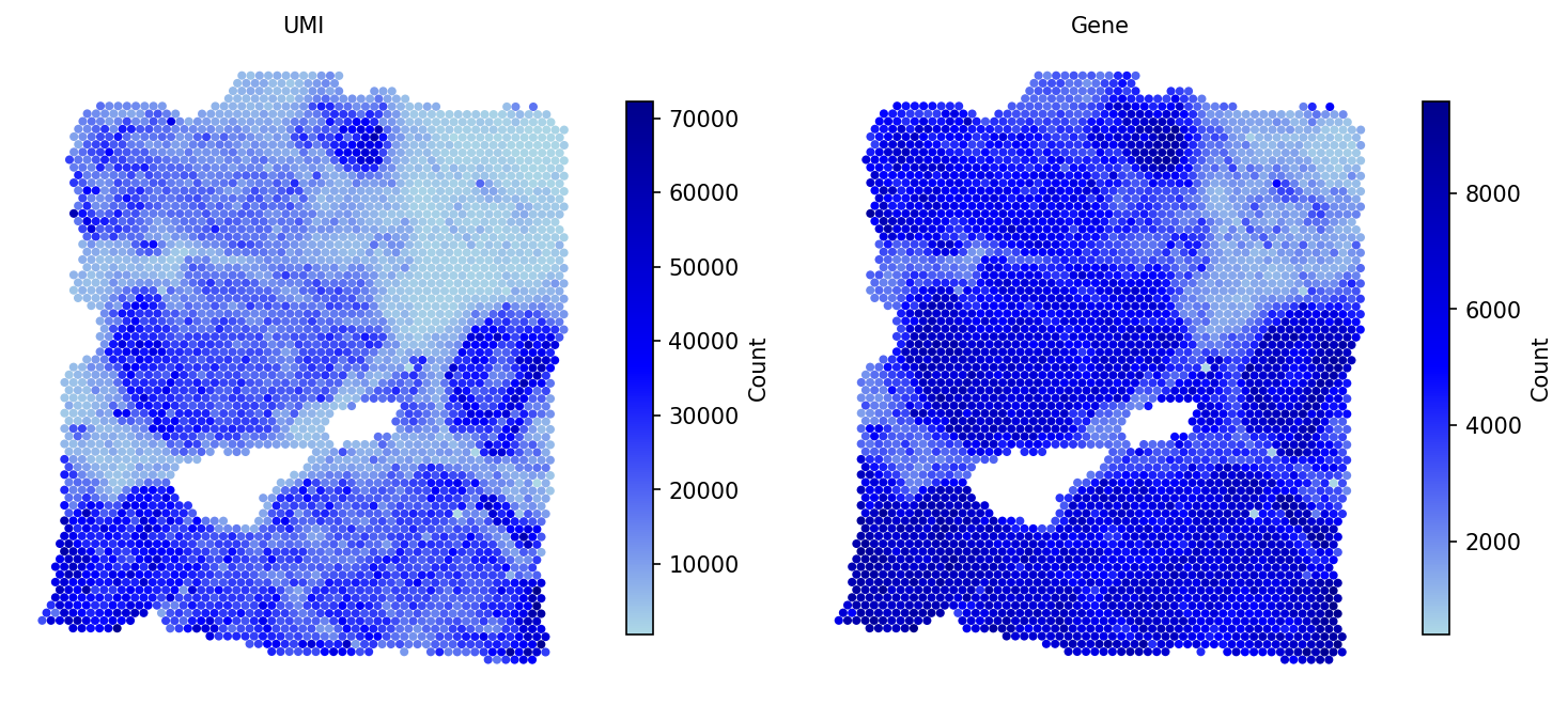
After QC, the metrics adata.obs['UMI'] and adata.obs['Gene'] are available for downstream analysis.

3. Deconvolve ST Data

Decompose each spot into cell-type fractions using the two-stage SpaCET algorithm. Stage 1 infers the malignant cell fraction using a gene pattern dictionary of copy number alterations (CNA) and expression changes specific to each cancer type. Stage 2 applies a constrained regression model based on hierarchical cell lineage to determine immune and stromal fractions.

# Run two-stage deconvolution for breast cancer (BRCA)
adata = spacet.deconvolution(adata, cancer_type="BRCA", n_jobs=5)

# View deconvolution results (cell types x spots)
prop_mat = adata.uns['spacet']['deconvolution']['propMat']
print(prop_mat.iloc[:13, :6])

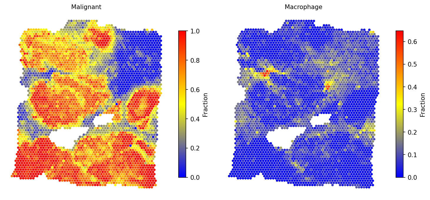
4. Visualize Cell Type Proportions

4a. Selected cell types

# Spatial distribution of selected cell types
spacet.visualize_spatial_feature(
    adata,
    spatial_type="CellFraction",
    spatial_features=["Malignant", "Macrophage"],
)

Spatial distribution of malignant and macrophage fractions. Color scale: blue (low) → yellow → red (high).

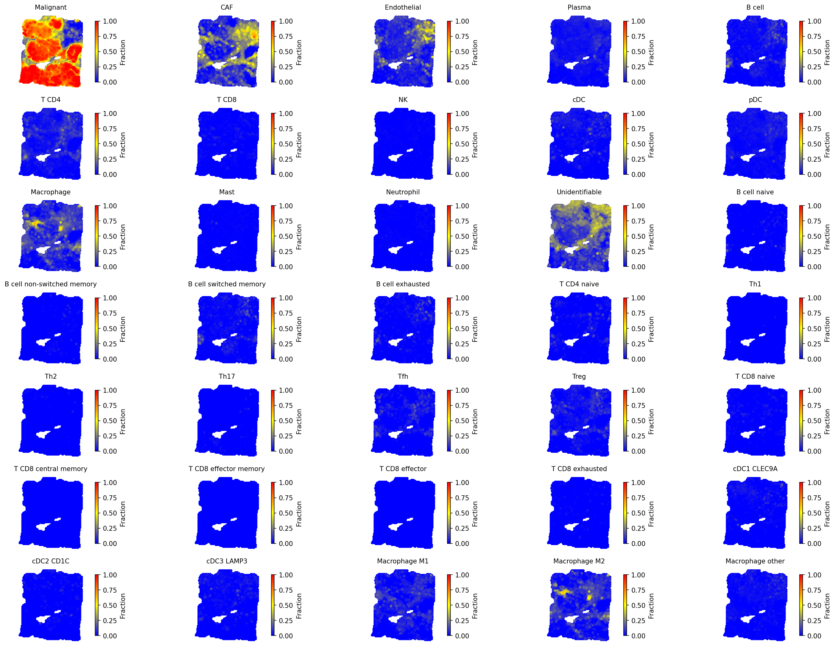
4b. All cell types

# Visualize all cell types with unified scale
spacet.visualize_spatial_feature(
    adata,
    spatial_type="CellFraction",
    spatial_features=["All"],
    same_scale_fraction=True,
    point_size=0.1,
    ncols=5,
)

Spatial distribution of all deconvolved cell types with unified [0, 1] color scale.

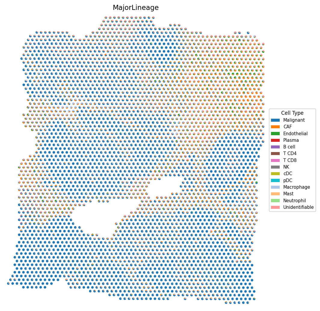
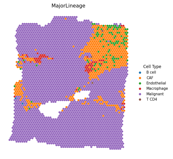
4c. Cell type composition (pie charts)

# Cell type composition as scatter pie charts
spacet.visualize_spatial_feature(
    adata,
    spatial_type="CellTypeComposition",
    spatial_features=["MajorLineage"],
    point_size=3,
)

Each spot displays a pie chart showing the relative proportions of major cell lineages (Malignant, CAF, Endothelial, Immune subtypes, Unidentifiable).

4d. Most abundant cell type

# Visualize the most abundant cell type per spot
spacet.visualize_spatial_feature(
    adata,
    spatial_type="MostAbundantCellType",
)

Each spot colored by its dominant cell type.

5. Estimate Cell-Cell Interactions

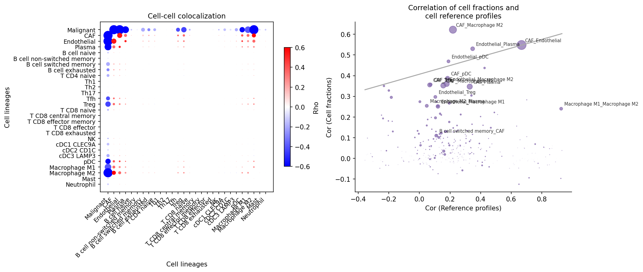
5a. Colocalization Analysis

Identify cell-type pairs that tend to colocalize. This analysis computes Spearman correlations of cell-type fractions across all spots. High positive correlations indicate colocalization tendency. The reference profile similarity is also computed to distinguish genuine interactions from transcriptomic similarity.

# Compute colocalization correlations
adata = spacet.cci_colocalization(adata)

# Visualize colocalization results
spacet.visualize_colocalization(adata)

Left: Correlation heatmap (red dots indicate colocalized pairs). Right: Comparison of fraction correlations vs. reference profile similarity. CAF–Macrophage M2 colocalization shows low profile similarity, indicating a genuine spatial interaction rather than transcriptomic similarity.

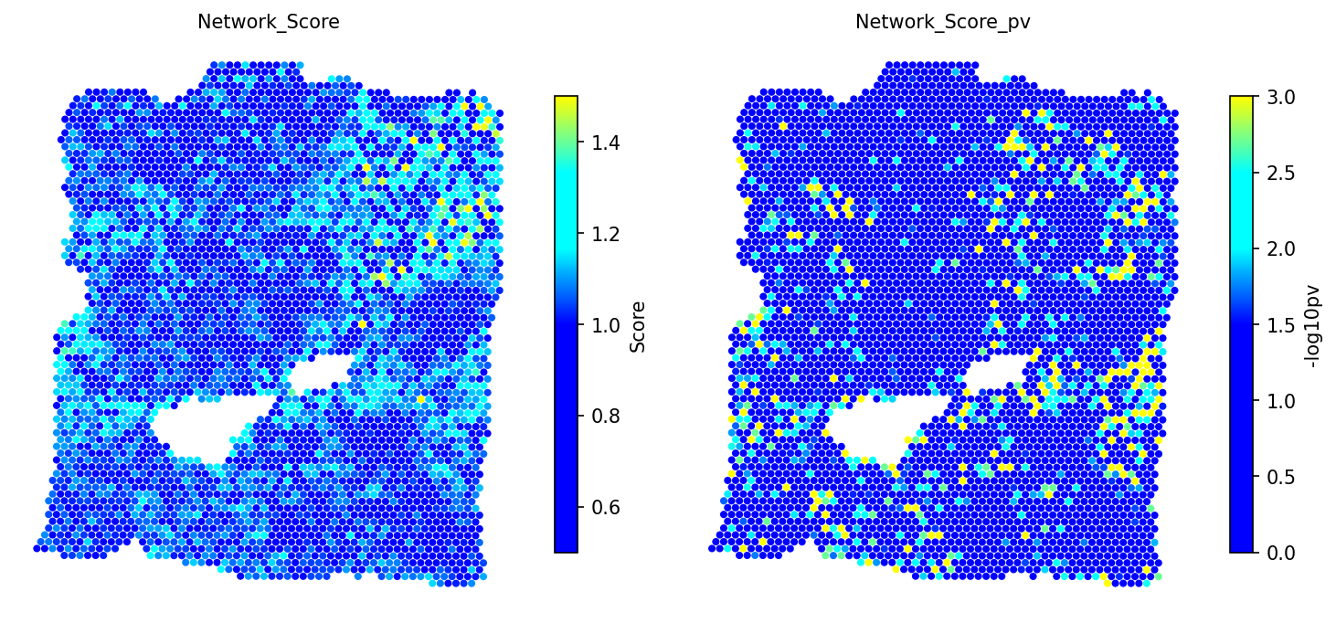
5b. Ligand-Receptor Network Score

Compute a ligand-receptor network score for each spot using an in-house database of ~2,500 L-R pairs. Significance is assessed by comparing against 1,000 BiRewire-based permuted networks that preserve directed degree distribution.

# Compute L-R network score with permutation testing
adata = spacet.cci_lr_network_score(adata, n_jobs=6)

# Visualize network scores and p-values
spacet.visualize_spatial_feature(
    adata,
    spatial_type="LRNetworkScore",
    spatial_features=["Network_Score", "Network_Score_pv"],
)

Spatial distribution of L-R network scores and their permutation-based p-values.

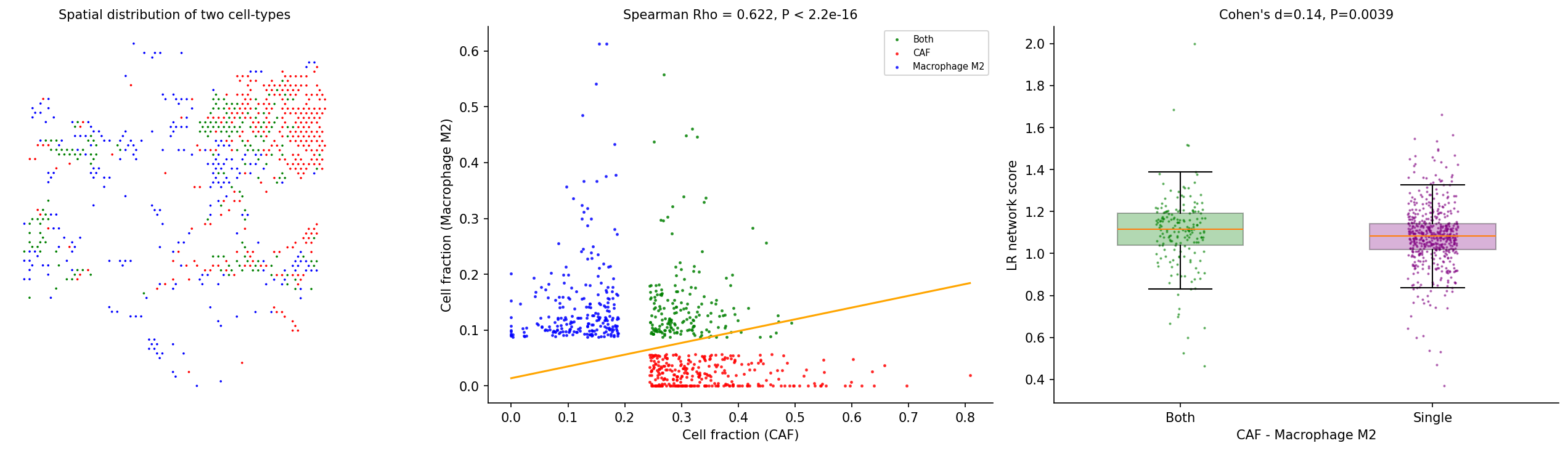
5c. Cell-Type Pair Enrichment

Test whether a colocalized cell-type pair has enriched L-R interactions. Spots are grouped into four categories: colocalized (high in both cell types), single-type dominated (high in one), or other. Cohen's d and Wilcoxon test assess whether colocalized spots have higher L-R network scores.

# Test CAF - Macrophage M2 interaction
adata = spacet.cci_cell_type_pair(
    adata,
    cell_type_pair=("CAF", "Macrophage M2"),
)

# Visualize the interaction analysis
spacet.visualize_cell_type_pair(
    adata,
    cell_type_pair=("CAF", "Macrophage M2"),
)

Three-panel visualization comparing L-R network scores across spot categories for the CAF–Macrophage M2 cell-type pair.

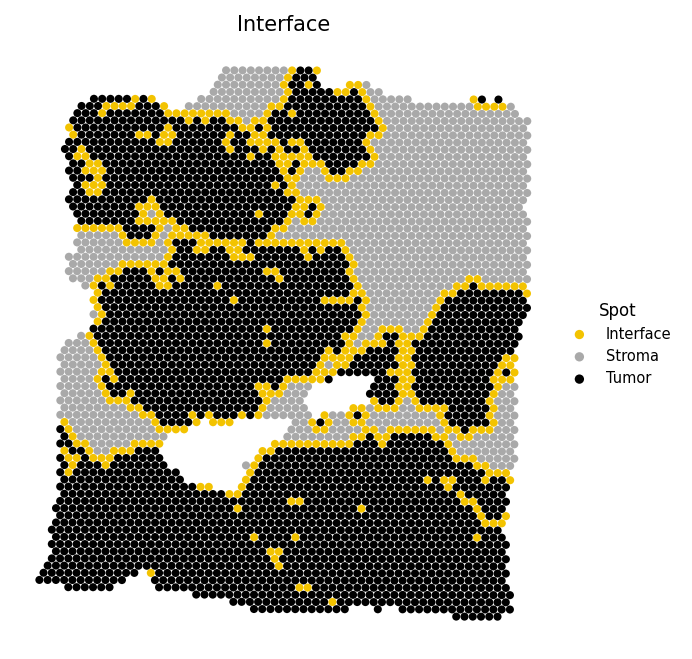
6. Tumor-Immune Interface Analysis

Identify spots at the tumor-stroma boundary and test whether cell-cell interactions cluster near this interface. Spots are classified as Tumor (malignant fraction ≥ 0.5), Interface (non-tumor with at least one tumor neighbor), or Stroma (non-tumor with no tumor neighbors).

6a. Identify interface

# Identify tumor-stroma interface spots
adata = spacet.identify_interface(adata)

# Visualize the interface
spacet.visualize_spatial_feature(
    adata,
    spatial_type="Interface",
    spatial_features=["Interface"],
)

Spatial classification of spots into Tumor, Stroma, and Interface regions.

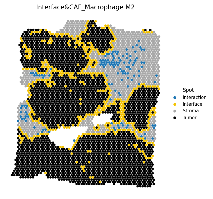
6b. Combine interface with interaction spots

# Overlay CAF-M2 interaction spots onto the interface map
adata = spacet.combine_interface(
    adata,
    cell_type_pair=("CAF", "Macrophage M2"),
)

# Visualize interface with interaction spots
spacet.visualize_spatial_feature(
    adata,
    spatial_type="Interface",
    spatial_features=["Interface&CAF_Macrophage M2"],
)

Interface map with CAF–Macrophage M2 interaction spots (green) overlaid on the tumor-stroma boundary.

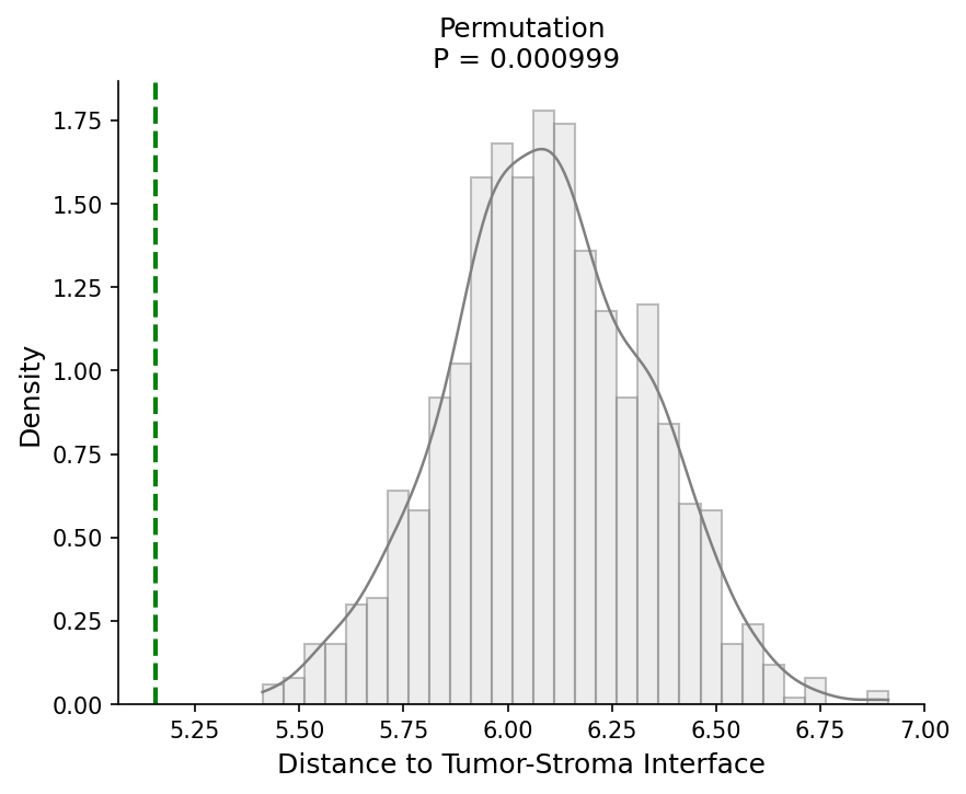
6c. Distance to interface

# Test if interaction spots are closer to the tumor border
adata = spacet.distance_to_interface(
    adata,
    cell_type_pair=("CAF", "Macrophage M2"),
)

# Visualize distance-to-interface permutation test
spacet.visualize_distance_to_interface(
    adata,
    cell_type_pair=("CAF", "Macrophage M2"),
)

Distance-to-interface permutation test. The observed mean distance from interaction spots to the nearest interface spot (red dashed line) is compared against 1,000 permutations of equal-sized random non-malignant spot sets.

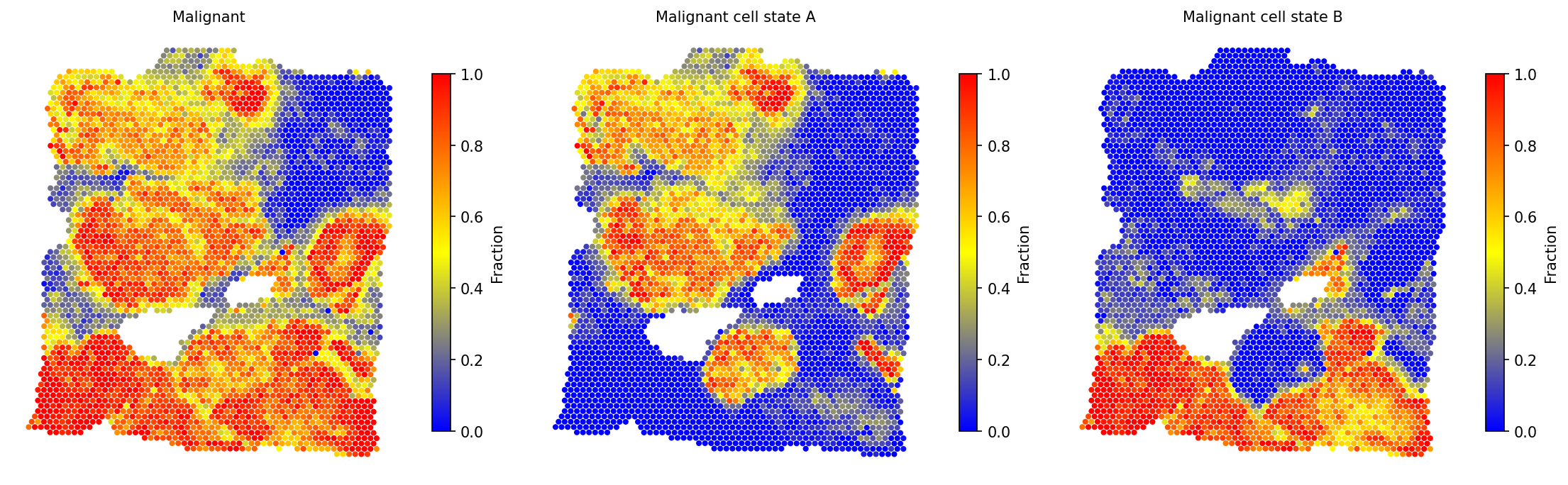
7. Explore Cancer Cell States

Characterize the spatial distribution of distinct malignant cell phenotypes. Spots with high malignant fraction (> 0.7) are clustered to discover sub-populations, and the malignant fraction is re-deconvolved into these states. Hierarchical clustering with silhouette-based cluster selection identifies the optimal number of states.

# Discover malignant cell states and re-deconvolve
adata = spacet.deconvolution_malignant(adata, n_jobs=6)

# View new malignant state fractions
prop_mat = adata.uns['spacet']['deconvolution']['propMat']
print(prop_mat.loc[
    ["Malignant cell state A", "Malignant cell state B"],
    prop_mat.columns[:6]
])

# Visualize malignant states alongside total malignant fraction
spacet.visualize_spatial_feature(
    adata,
    spatial_type="CellFraction",
    spatial_features=[
        "Malignant",
        "Malignant cell state A",
        "Malignant cell state B",
    ],
    ncols=3,
)

Spatial distribution of total malignant fraction and individual malignant cell states. Cell state fractions sum to the total malignant fraction per spot.

Session Info

import spatialgpu
print(f"spatial-gpu version: {spatialgpu.__version__}")

import anndata, numpy, scipy, pandas, matplotlib
print(f"anndata:     {anndata.__version__}")
print(f"numpy:       {numpy.__version__}")
print(f"scipy:       {scipy.__version__}")
print(f"pandas:      {pandas.__version__}")
print(f"matplotlib:  {matplotlib.__version__}")

try:
    import cupy
    print(f"cupy:        {cupy.__version__} (GPU backend available)")
except ImportError:
    print("cupy:        not installed (CPU-only mode)")