Cell-cell communication for single-cell resolution spatial transcriptomics data

Adapted from the SecAct R tutorial using the spatial-gpu package

This tutorial demonstrates inference of cell-cell communication mediated by secreted proteins from single-cell resolution spatial transcriptomics data. The demonstration uses a liver cancer sample from the CosMx platform.

1. Read ST data to a SpaCET object

To load data, users can create a SpaCET object by preparing three types of input data:

1. Count data (matrix format: genes × cell IDs)
2. Spatial location information (matrix format: cell IDs × coordinates, X and Y columns)
3. Meta data, optional (matrix format: cell IDs × annotations)

import spatialgpu.deconvolution as spacet
import anndata as ad

# Load CosMx LIHC data
# Download from: https://zenodo.org/records/15006880
adata = ad.read_h5ad("data/LIHC_CosMx/LIHC_CosMx.h5ad")

# Show count matrix dimensions
print(adata.shape)

# Show coordinate matrix
print(adata.obs[["coordinate_x_um", "coordinate_y_um"]].head())

# Show meta information
print(adata.obs[["cellType", "niche"]].head())

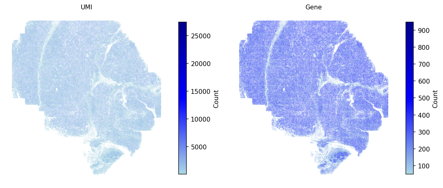
# Filter out cells with less than 50 expressed genes
adata = spacet.quality_control(adata, min_genes=50)

# Plot the QC metrics
spacet.visualize_spatial_feature(
    adata,
    spatial_type="QualityControl",
    spatial_features=["UMI", "Gene"],
    point_size=0.1,
)

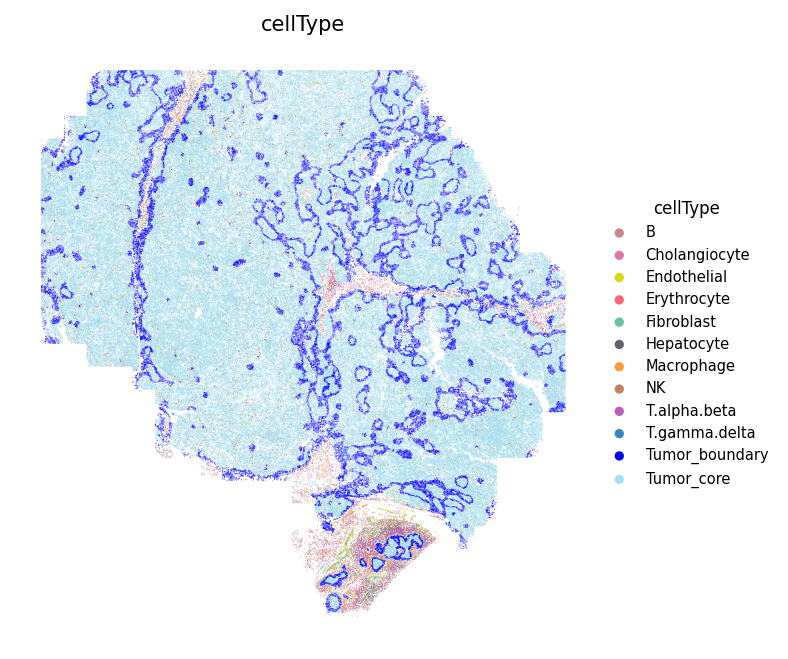
The SpaCET object contains cell type annotations from the original study. Display the spatial distribution of all cell types:

# Define cell type colors
cell_colors = {
    'B': '#C88888',
    'Erythrocyte': '#fe666d',
    'T.alpha.beta': '#B95FBB',
    'T.gamma.delta': '#3288bd',
    'NK': '#bb8761',
    'Hepatocyte': '#63636d',
    'Cholangiocyte': '#de77ae',
    'Endothelial': '#D4D915',
    'Fibroblast': '#66c2a5',
    'Macrophage': '#ff9a36',
    'Tumor_core': '#A4DFF2',
    'Tumor_boundary': 'blue',
    'Other': '#cccccc',
}

# Show the spatial distribution of all cell types
spacet.visualize_spatial_feature(
    adata,
    spatial_type="metaData",
    spatial_features=["cellType"],
    colors=cell_colors,
    point_size=0.1,
)

2. Infer secreted protein activity

After loading ST data, users run secact_inference() to infer signaling activities of secreted proteins for each cell. Output stored in adata.uns['spacet']['SecAct_output']['SecretedProteinActivity'] contains four items: beta (regression coefficients), se (standard error), zscore (beta/se), and pvalue (two-sided test p-value from permutation test).

# Infer activity; ~30 mins
adata = spacet.secact_inference(
    adata,
    scale_factor=1000,
)

# Show activity
zscores = adata.uns['spacet']['SecAct_output']['SecretedProteinActivity']['zscore']
print(zscores.iloc[:6, :3])

3. Infer cell-cell communication

After calculating the secreted protein activity, SecAct estimates cell-cell communication mediated by secreted proteins. This module contains two steps.

First, SecAct filters >1,000 secreted proteins to identify significant ones mediating intercellular communication by calculating Spearman correlation between protein signaling activity and neighbor cells’ sum expression. P values are adjusted by Benjamini-Hochberg (BH) method as false discovery rate (FDR). Cutoffs: r > 0.05 and FDR < 0.01.

Second, for each secreted protein, SecAct statistically tests whether it mediates communication between cell types. Neighboring pairs of cells are identified where distance < 20 μm. A communicating pair requires the sender expressing the protein RNA (count > 0) and the receiver showing signaling activity (score > 0). The communication score is defined as the ratio of communicating pairs to total neighboring pairs. P-value is computed through 1,000 randomizations with cell IDs permuted within each type (Benjamini–Hochberg adjusted). Significant if ratio > 0.2 and FDR < 0.01.

# Infer CCC; ~20 mins
adata = spacet.secact_spatial_ccc(
    adata,
    cell_type_col="cellType",
    scale_factor=1000,
    radius=20,
    ratio_cutoff=0.2,
    padj_cutoff=0.01,
)

# Show output
ccc = adata.uns['spacet']['SecAct_output']['SecretedProteinCCC']
print(ccc.head())

4. Visualize cell-cell communication

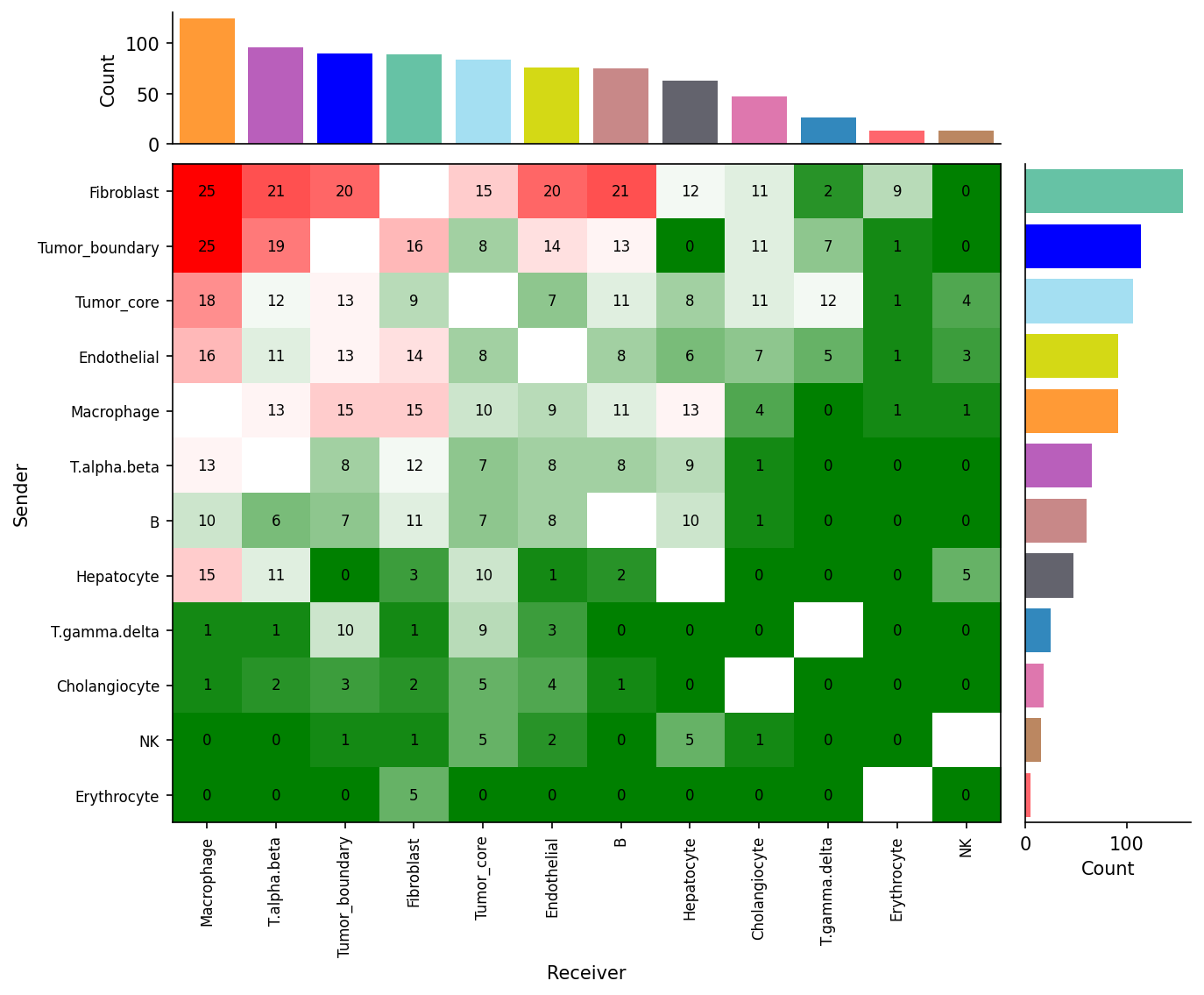
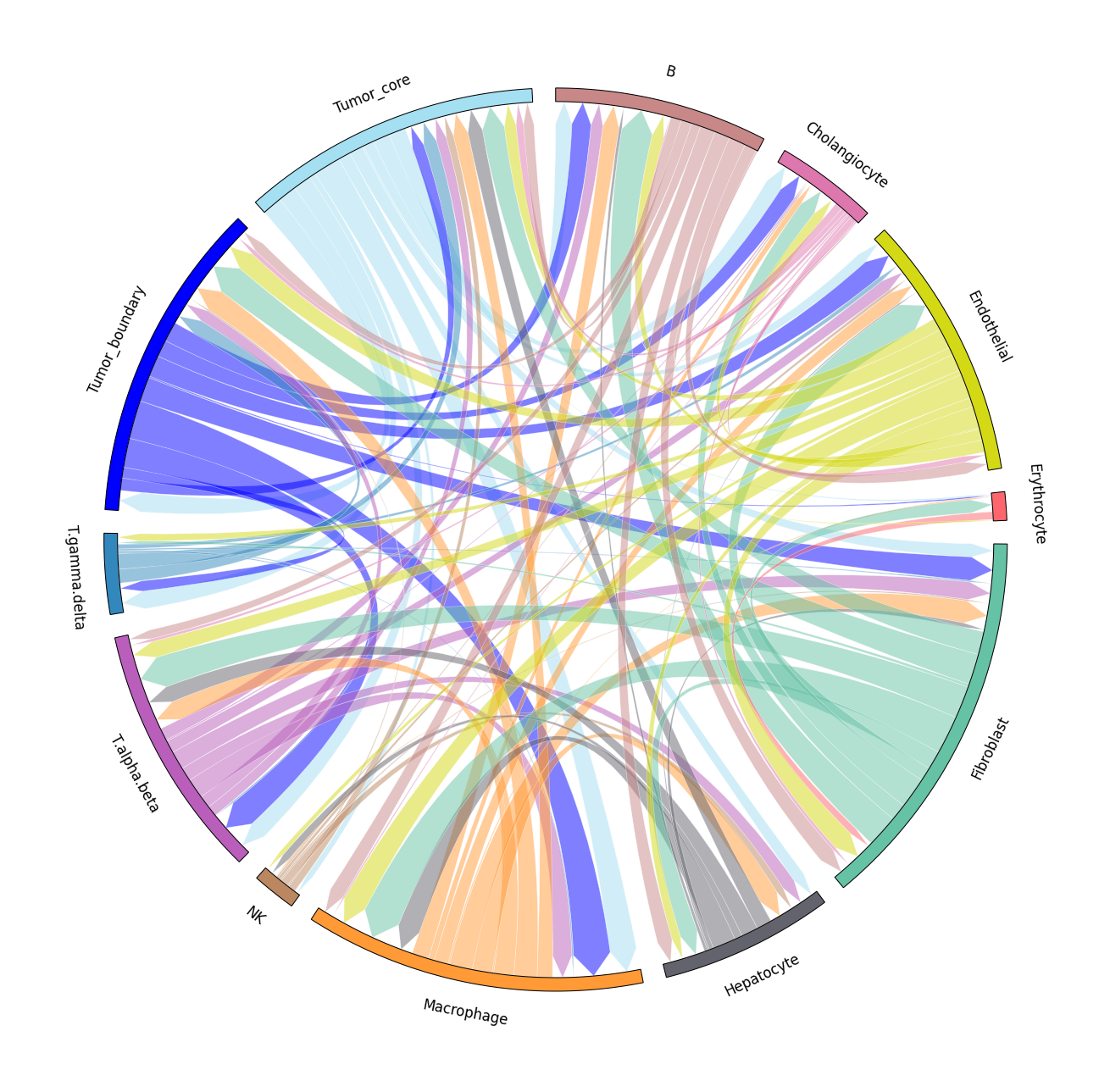
We provide two types of visualization: heatmap and circle plot. The number in the heatmap represents the count of secreted proteins from senders to receivers.

spacet.visualize_secact_heatmap(
    adata,
    row_sorted=True,
    column_sorted=True,
    colors_cell_type=cell_colors,
)

spacet.visualize_secact_circle(
    adata,
    colors_cell_type=cell_colors,
)

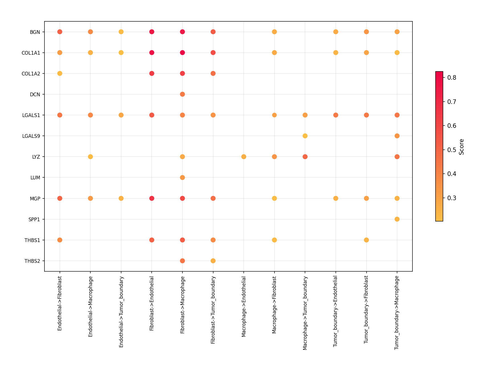
Users can select specific cell-cell communication from adata.uns['spacet']['SecAct_output']['SecretedProteinCCC'] to visualize. The visualize_secact_dotplot() function requires sender, secreted_protein, and receiver parameters.

cell_types = ["Tumor_boundary", "Fibroblast", "Macrophage", "Endothelial"]

proteins = [
    "BGN", "COL1A1", "COL1A2", "DCN", "IGFBP5",
    "LGALS1", "LGALS9", "LYZ", "LUM", "MGP",
    "SPP1", "THBS1", "THBS2",
]

spacet.visualize_secact_dotplot(
    adata,
    sender=cell_types,
    secreted_protein=proteins,
    receiver=cell_types,
)

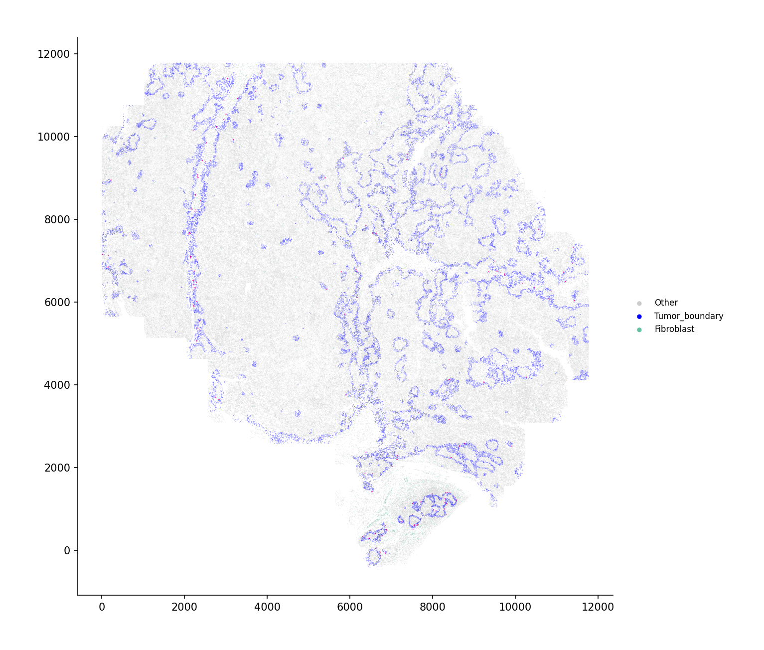
5. Visualize secreted signaling velocity

Users can select specific communications from adata.uns['spacet']['SecAct_output']['SecretedProteinCCC'] to visualize using visualize_secact_velocity_scst(). Assignment of values to sender, secreted_protein, and receiver is required.

# Compute single-cell resolution velocity
vel = spacet.secact_signaling_velocity_scst(
    adata,
    sender="Fibroblast",
    secreted_protein="THBS2",
    receiver="Tumor_boundary",
    cell_type_col="cellType",
)

# Full view
spacet.visualize_secact_velocity_scst(
    vel,
    show_coordinates=True,
    colors=cell_colors,
    point_size=0.1,
    legend_position="right",
    legend_size=2,
    arrow_color="#ff0099",
    arrow_size=1.0,
    arrow_width=0.5,
)

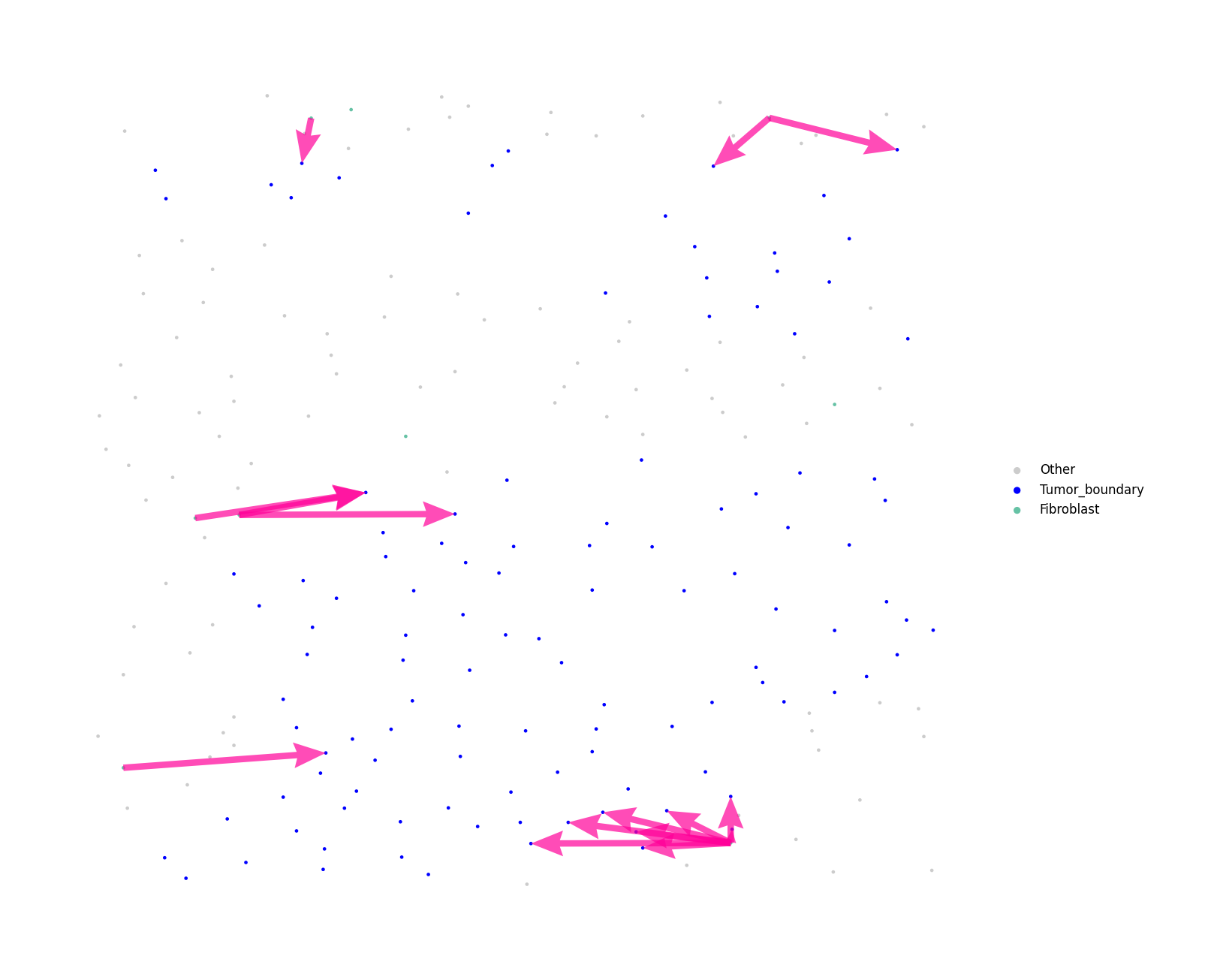
# Zoomed view
spacet.visualize_secact_velocity_scst(
    vel,
    customized_area=[8290, 8366, 1100, 1400],
    show_coordinates=False,
    colors=cell_colors,
    point_size=15,
    legend_position="right",
    legend_size=3,
    arrow_color="#ff0099",
    arrow_size=0.3,
    arrow_width=0.5,
)

For large datasets, use interactive=True to get a zoomable plotly figure instead of a static image:

# Interactive zoomable view (plotly)
fig = spacet.visualize_secact_velocity_scst(
    vel,
    interactive=True,
    colors=cell_colors,
    point_size=2,
    arrow_color="#ff0099",
    arrow_size=3.0,
    arrow_width=1.5,
    save="velocity_interactive.html",
)