Cell Type Deconvolution for Old ST Pancreatic Ductal Adenocarcinoma

Python GPU-accelerated Adapted from the SpaCET R tutorial for pancreatic ductal adenocarcinoma with matched scRNA-seq

Overview

This tutorial demonstrates how to use spatial-gpu to deconvolve spatial transcriptomics data from a pancreatic ductal adenocarcinoma (PDAC) sample profiled on the "oldST" platform (Moncada et al., 2020). Each spot has a diameter of approximately 100 μm, capturing multiple cells per spot.

Unlike the Visium breast cancer tutorial which uses built-in reference signatures, this tutorial uses a matched scRNA-seq reference dataset from the same tumor for deconvolution. The matched reference provides a lineage tree describing the hierarchical relationship among cell types, enabling more accurate cell fraction estimation.

The spatial-gpu package provides a GPU-accelerated Python implementation of the SpaCET algorithm (Nature Communications 14, 568, 2023). All functions work on AnnData objects and store results in adata.uns['spacet'].

API Mapping: R SpaCET → spatial-gpu

1. Create SpaCET Object

Load the oldST PDAC spatial transcriptomics data into an AnnData object. The dataset contains a counts matrix and spot coordinates from the original spatial transcriptomics platform.

import spatialgpu.deconvolution as spacet
import anndata as ad

# Load ST data from h5ad file
adata = ad.read_h5ad("data/oldST_PDAC/st_PDAC.h5ad")

# Inspect the object
print(adata)

2. Load scRNA-seq Reference

Load the matched single-cell RNA-seq reference dataset and the associated cell lineage tree. The lineage tree defines the hierarchical relationships among cell types and is required for the matched scRNA-seq deconvolution algorithm.

# Load matched scRNA-seq reference data
sc_adata = ad.read_h5ad("data/oldST_PDAC/sc_PDAC.h5ad")

# Extract the lineage tree from the reference
lineage_tree = sc_adata.uns["lineage_tree"]

# Inspect the reference
print(sc_adata)
print("Cell types:", sc_adata.obs["cell_type"].unique().tolist())
print("Lineage tree:", lineage_tree)

3. Deconvolve with Matched scRNA-seq

Run the matched scRNA-seq deconvolution algorithm. This method uses the single-cell reference profiles and lineage tree to estimate cell-type fractions at each spot via hierarchical constrained regression.

import pandas as pd

# Prepare scRNA-seq inputs (counts, annotation, lineage tree)
# sc_counts: genes x cells DataFrame
sc_counts = pd.DataFrame(
    sc_adata.X.toarray().T if hasattr(sc_adata.X, 'toarray') else sc_adata.X.T,
    index=sc_adata.var_names,
    columns=sc_adata.obs_names,
)

# sc_annotation: DataFrame with 'cellID' and 'cellType' columns
sc_annotation = pd.DataFrame({
    "cellID": sc_adata.obs_names,
    "cellType": sc_adata.obs["cell_type"].values,
})

# Deconvolve using matched scRNA-seq reference
adata = spacet.deconvolution_matched_scrnaseq(
    adata,
    sc_counts=sc_counts,
    sc_annotation=sc_annotation,
    sc_lineage_tree=lineage_tree,
    n_jobs=6,
)

# View deconvolution results (cell types x spots)
prop_mat = adata.uns['spacet']['deconvolution']['propMat']
print(prop_mat.iloc[:, :5])

4. Visualize Results

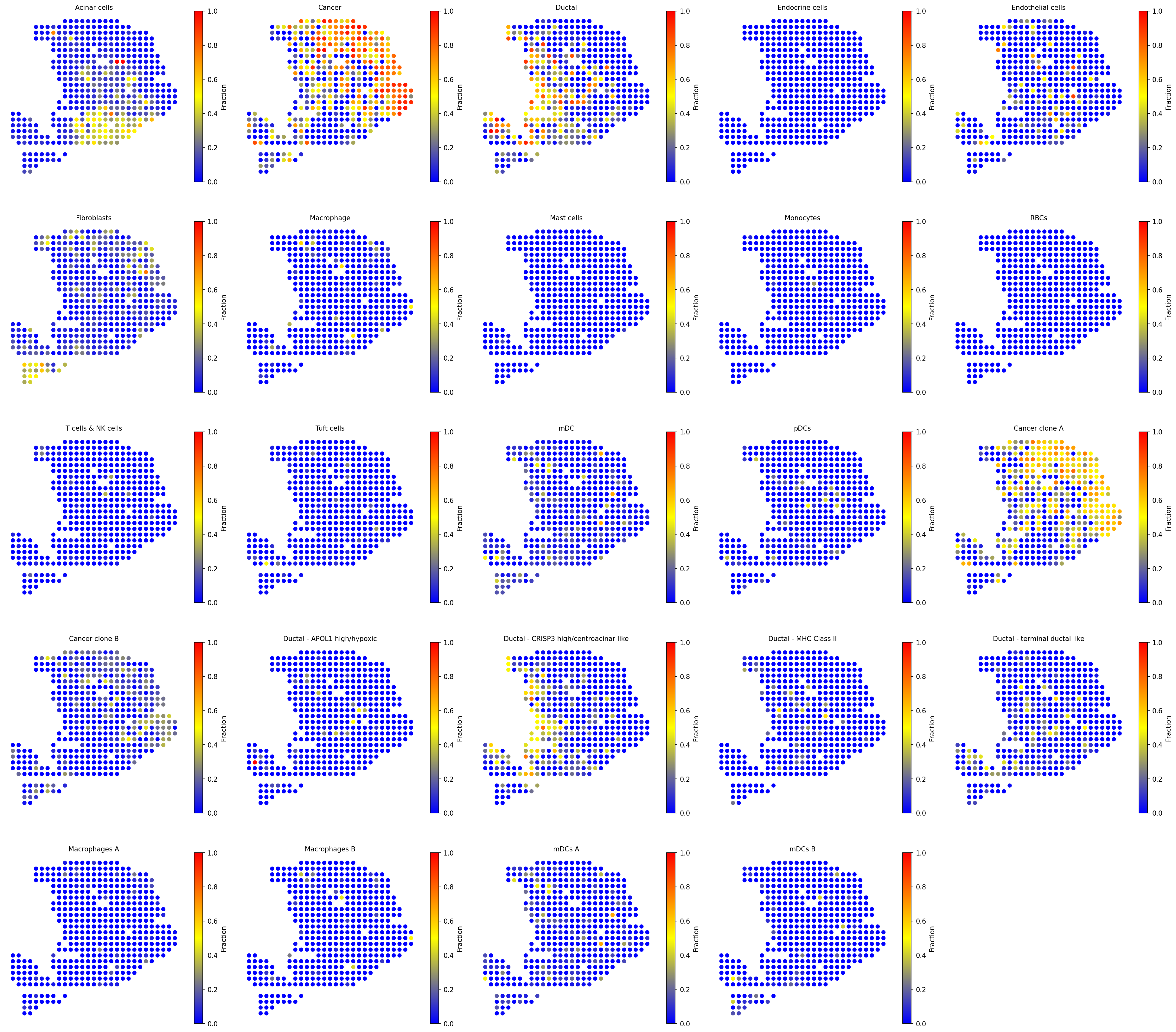
4a. All cell types

Visualize the spatial distribution of all deconvolved cell-type fractions with a unified color scale across panels.

# Visualize all cell type fractions with unified scale
spacet.visualize_spatial_feature(
    adata,
    spatial_type="CellFraction",
    spatial_features=["All"],
    same_scale_fraction=True,
    point_size=1.5,
    ncols=5,
)

Spatial distribution of all deconvolved cell types with unified [0, 1] color scale. Cancer clones A and B occupy distinct spatial regions of the tumor.

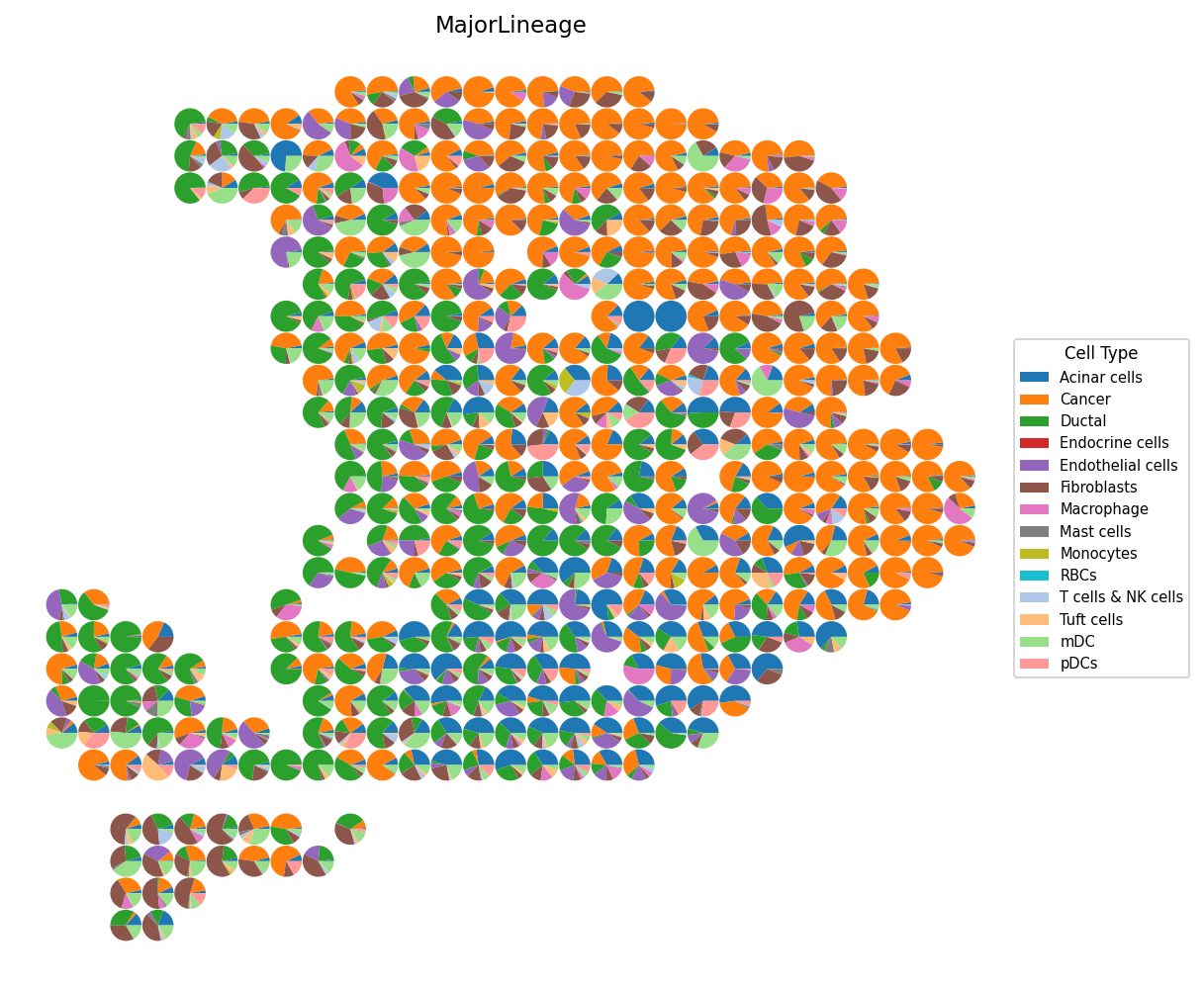
4b. Cell type composition (pie charts)

# Cell type composition as scatter pie charts
spacet.visualize_spatial_feature(
    adata,
    spatial_type="CellTypeComposition",
    spatial_features=["MajorLineage"],
    point_size=0.5,
)

Each spot displays a pie chart showing the relative proportions of major cell lineages. Cancer clones, Ductal subtypes, and Acinar cells dominate different spatial regions.

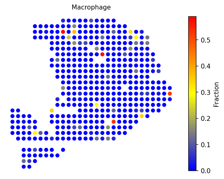
4c. Specific cell types

Examine individual cell types of interest, including cancer clones and tissue-specific cell populations.

# Visualize specific cell types
spacet.visualize_spatial_feature(
    adata,
    spatial_type="CellFraction",
    spatial_features=["Cancer clone A", "Cancer clone B",
                       "Acinar cells", "Ductal - CRISP3 high/centroacinar like"],
    ncols=2,
)

Spatial distribution of selected cell types. Cancer clone A and B show distinct spatial patterns, while Acinar and Ductal-CRISP3 cells localize to specific tissue regions.

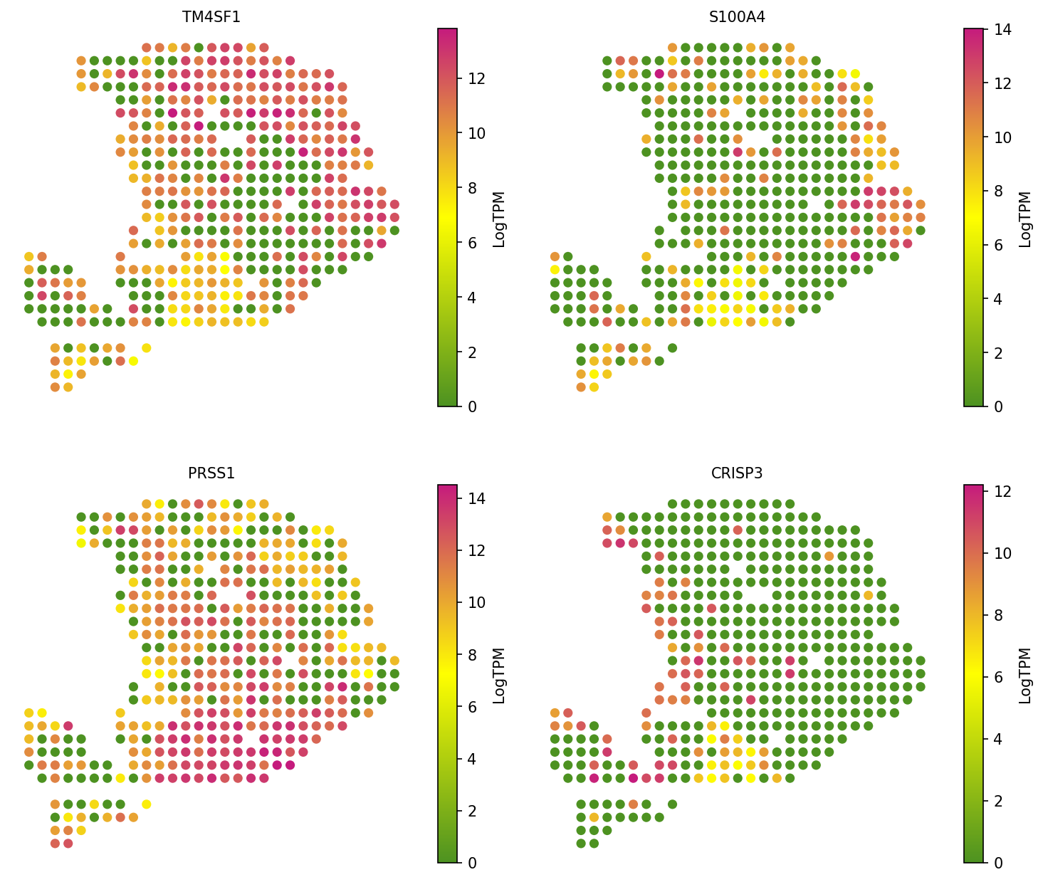
4d. Gene expression validation

Validate the deconvolution results by visualizing marker gene expression. Each gene should show spatial concordance with its associated cell type.

# Visualize marker gene expression for validation
spacet.visualize_spatial_feature(
    adata,
    spatial_type="GeneExpression",
    spatial_features=["TM4SF1", "S100A4", "PRSS1", "CRISP3"],
    ncols=2,
)

Spatial expression of marker genes: TM4SF1 (Cancer), S100A4 (Fibroblast/Macrophage), PRSS1 (Acinar), CRISP3 (Ductal-CRISP3). Expression patterns validate the deconvolution results.

Session Info

import spatialgpu
print(f"spatial-gpu version: {spatialgpu.__version__}")

import anndata, numpy, scipy, pandas, matplotlib
print(f"anndata:     {anndata.__version__}")
print(f"numpy:       {numpy.__version__}")
print(f"scipy:       {scipy.__version__}")
print(f"pandas:      {pandas.__version__}")
print(f"matplotlib:  {matplotlib.__version__}")

try:
    import cupy
    print(f"cupy:        {cupy.__version__} (GPU backend available)")
except ImportError:
    print("cupy:        not installed (CPU-only mode)")